Replicate a figure from an article

In one course I give, students are asked to review a scientific article (a clinical trial in cancerology).

These same students have an R programming course with me later on, so I thought: what if the course content was to reproduce some of the figures in the study?

This would be interesting, educationally speaking, but the data from the clinical trial is obviously not available.

So here I am, trying to simulate data so that it gives results similar to those in the article.

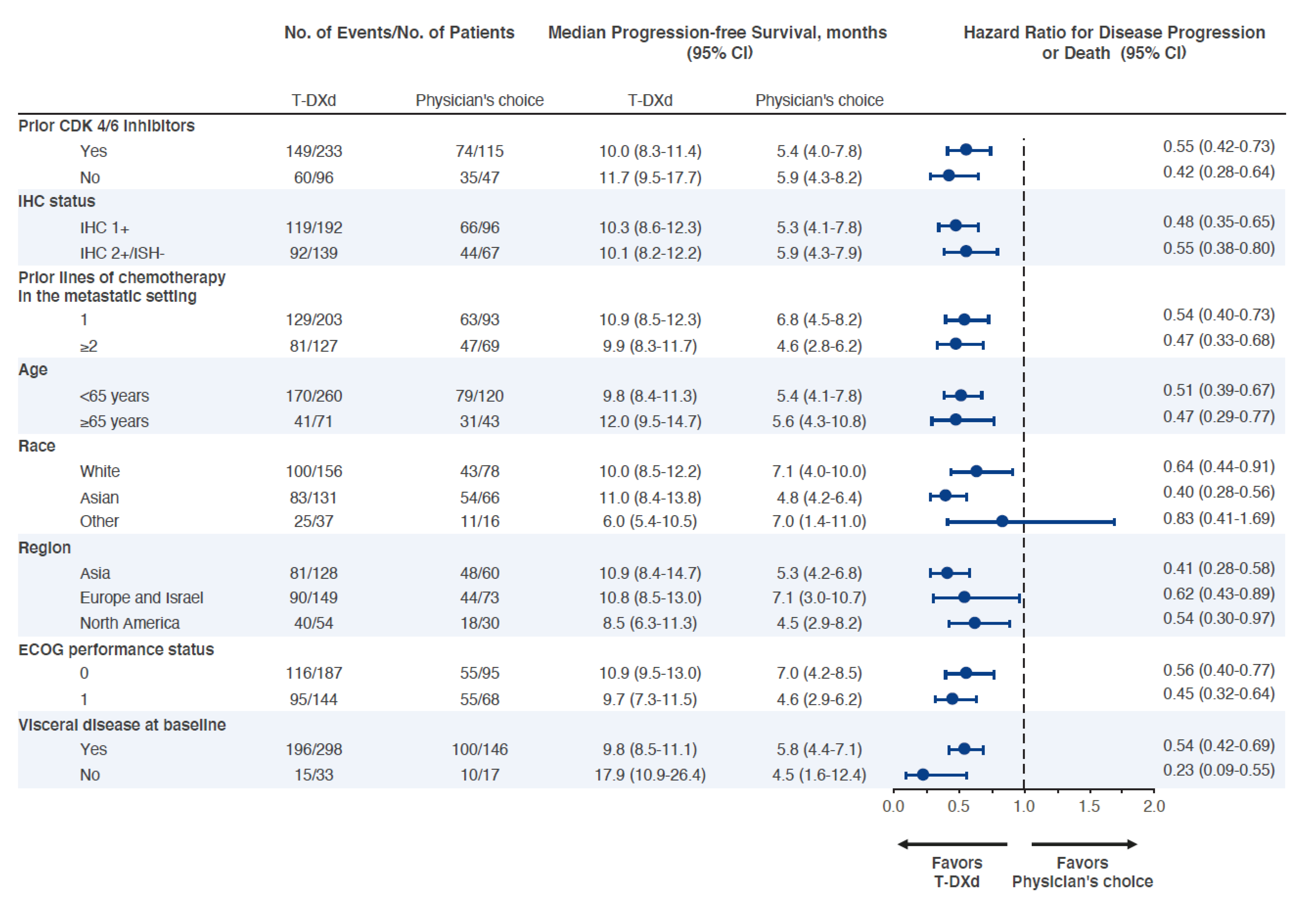
The article (open-access), “Trastuzumab Deruxtecan in Previously Treated HER2-Low Advanced Breast Cancer”, is about a phase 3 clinical trial testing the Progression-Free Survival of patients assigned to Trastuzumab Deruxtecan or another chemotherapy.

Scrape data from the article ♻️

If I want to replicate the article, I will need some input data. The Figure S2 (Appendix, page 15) is perfect for that, and I think it will be the perfect figure for my course. Let’s scrape it!

Figure S2 from https://doi.org/10.1056/NEJMoa2203690

Init

Here are the packages I will be using:

library(tidyverse)
library(survival)
library(ggsurvfit)
library(patchwork)

Baseline Data

First, I manually entered all the labels and sample sizes of all the covariates in sample() to generate a simulated population with the right baseline data.

As this implies some randomness, I encapsulate the process in the get_data() function and set the seed (more on that later).

#' Recreate article's baseline data
#' Data is from table S2 number of patients (`no_patients_tx` and `no_events_pc`)
get_data = function(){
  f = function(lvl, nb) sample(rep(lvl, nb)) |> fct_relevel(lvl[1])
  df0 = tibble(
    id = factor(1:331),
    arm = "T-DXd",
    age = f(c("<65 years", "\U{2265}65 years"), c(260, 71)),
    race = f(c("White", "Asian", "Other", NA), c(156, 131, 37, 7)),
    region = f(c("Asia", "Europe and Israel", "North America"), c(128, 149, 54)),
    ecog = f(c("0", "1"), c(187, 144)),
    prior_cdki = f(c("Yes", "No", NA), c(233, 96, 2)),
    prior_lines = f(c("1", "\U{2265}2", NA), c(203, 127, 1)),
    ihc = f(c("IHC 1+", "IHC 2+/ISH-"), c(192, 139)),
    visceral_bl = f(c("Yes", "No"), c(298, 33)),
  )
  
  df1 = tibble(
    id = factor(331+c(1:163)),
    arm = "Physician's choice",
    age = f(c("<65 years", "\U{2265}65 years"), c(120, 43)),
    race = f(c("White", "Asian", "Other", NA), c(78, 66, 16, 3)),
    region = f(c("Asia", "Europe and Israel", "North America"), c(60, 73, 30)),
    ecog = f(c("0", "1"), c(95, 68)),
    prior_cdki = f(c("Yes", "No", NA), c(115, 47, 1)),
    prior_lines = f(c("1", "\U{2265}2", NA), c(93, 69, 1)),
    ihc = f(c("IHC 1+", "IHC 2+/ISH-"), c(96, 67)),
    visceral_bl = f(c("Yes", "No"), c(146, 17)),
  )
  
  bind_rows(df0, df1) |> 
    mutate(
      arm = fct_relevel(arm, "Physician's choice"),
      prior_cdki = fct_relevel(prior_cdki, "Yes"),
      ihc = fct_relevel(ihc, "IHC 1+"),
      prior_lines = fct_relevel(prior_lines, "1"),
      age = fct_relevel(age, "<65 years"),
      race = fct_relevel(race, "White", "Asian"),
      region = fct_relevel(region, "Asia", "Europe and Israel"),
      ecog = fct_relevel(ecog, "0"),
      visceral_bl = fct_relevel(visceral_bl, "Yes"),
    ) |> 
    crosstable::apply_labels(
      prior_cdki = "Prior CDK 4/6 inhibitors", ihc = "IHC status",
      prior_lines = "Prior lines of chemotherapy in the metastatic setting",
      age = "Age", race = "Race", region = "Region", ecog = "ECOG performance status",
      visceral_bl = "Visceral disease at baseline"
    )
}

set.seed(517)
data_baseline = get_data()
data_baseline

Coefficients Data

Bored to death by the first step, I changed strategy and directly fed ChatGPT-4o with figure S2, asking for an R dataframe containing the data. The result was nearly perfect, but I used constructive::construct() to improve the readability.

data_figS2 = tibble(
  variable = rep(
    c(
      "Prior CDK 4/6 inhibitors", "IHC status",
      "Prior lines of chemotherapy in the metastatic setting", "Age", "Race",
      "Region", "ECOG performance status", "Visceral disease at baseline"
    ),
    rep(c(2L, 3L, 2L), c(4L, 2L, 2L))
  ),
  variable_key = rep(
    c("prior_cdki", "ihc", "prior_lines", "age", "race", "region", "ecog", "visceral_bl"),
    rep(c(2L, 3L, 2L), c(4L, 2L, 2L))
  ),
  level = c(
    "Yes", "No", "IHC 1+", "IHC 2+/ISH-", "1", "\U{2265}2", "<65 years",
    "\U{2265}65 years", "White", "Asian", "Other", "Asia", "Europe and Israel",
    "North America", "0", "1", "Yes", "No"
  ),
  no_events_tx = c(149, 60, 119, 92, 129, 81, 170, 41, 100, 33, 25, 81, 90, 36, 116, 80, 196, 15),
  no_patients_tx = c(233, 95, 192, 139, 203, 127, 260, 51, 156, 54, 37, 128, 149, 48, 187, 146, 298, 33),
  no_events_pc = c(74, 35, 46, 44, 63, 39, 79, 21, 45, 18, 11, 82, 94, 40, 55, 58, 108, 15),
  no_patients_pc = c(115, 47, 65, 66, 103, 72, 121, 29, 102, 40, 16, 128, 147, 48, 87, 91, 122, 16),
  median_pfs_tx = c(10, 11.7, 10.8, 10.1, 10.9, 9.3, 9.8, 9.4, 10.5, 11, 9.6, 10.1, 9.8, 10.2, 9.8, 10, 9.8, 10.1),
  ci_pfs_tx = c(
    "8.3-11.4", "9.6-13.1", "8.6-12.3", "8.2-12.2", "8.5-12.5", "8.1-12.0",
    "8.9-11.3", "7.4-11.7", "9.5-12.2", "7.8-NA", "7.4-NA", "8.3-11.9",
    "8.6-11.7", "8.4-NA", "8.8-11.1", "8.4-11.4", "9.8-11.1", "9.6-NA"
  ),
  median_pfs_pc = c(5.4, 5.9, 5.8, 6, 6.4, 6.8, 5.4, 5.8, 6.5, 5.7, 4, 5.7, 5.8, 5.6, 5.3, 6.1, 5.3, 5.7),
  ci_pfs_pc = c(
    "4.0-7.8", "4.8-7.2", "4.3-7.7", "3.9-7.9", "4.8-8.2", "4.5-8.2", "4.4-7.8",
    "4.1-10.4", "4.7-8.1", "3.9-10.6", "1.4-11.0", "4.3-7.8", "4.6-7.4",
    "3.4-8.1", "4.4-7.9", "4.5-7.8", "5.1-6.4", "5.6-NA"
  ),
  hr = c(
    0.55, 0.42, 0.48, 0.55, 0.54, 0.47, 0.51, 0.47, 0.64, 0.4, 0.83, 0.41, 0.62,
    0.54, 0.56, 0.45, 0.54, 0.23
  ),
  ci_inf = c(
    0.42, 0.28, 0.35, 0.38, 0.4, 0.33, 0.39, 0.29, 0.44, 0.28, 0.41, 0.28, 0.43,
    0.3, 0.4, 0.32, 0.42, 0.09
  ),
  ci_sup = c(
    0.73, 0.64, 0.65, 0.8, 0.73, 0.68, 0.67, 0.77, 0.91, 0.56, 1.69, 0.58, 0.89,
    0.97, 0.77, 0.64, 0.69, 0.55
  ),
)
data_coef = data_figS2 |> 
  select(variable_key, level, coef=hr, ci_inf, ci_sup) |>
  mutate(
    across(coef:ci_sup, log),
    se = abs(ci_inf-ci_sup)/2,
    coef_rel = coef-log(0.51)
  )

data_coef

Check ✔️

Let’s stop for a second and explore the baseline dataset that we generated.

Table 1

Did we reproduced the left side of Table 1 ?

Almost. There are differences, some most likely due to analytic reasons (e.g. missing data in race), and some that I don’t understand (e.g. prior lines of chemotherapy).

library(crosstable)
data_baseline |> 
  crosstable(c(region, race, ecog, prior_cdki, prior_lines), by=arm) |> 
  as_flextable(keep_id=TRUE)

	arm
	Physician's choice (N=163)	T-DXd (N=331)
Region (region)
Asia	60 (36.8%)	128 (38.7%)
Europe and Israel	73 (44.8%)	149 (45.0%)
North America	30 (18.4%)	54 (16.3%)
Race (race)
White	78 (48.8%)	156 (48.1%)
Asian	66 (41.2%)	131 (40.4%)
Other	16 (10.0%)	37 (11.4%)
NA	3	7
ECOG performance status (ecog)
0	95 (58.3%)	187 (56.5%)
1	68 (41.7%)	144 (43.5%)
Prior CDK 4/6 inhibitors (prior_cdki)
Yes	115 (71.0%)	233 (70.8%)
No	47 (29.0%)	96 (29.2%)
NA	1	2
Prior lines of chemotherapy in the metastatic setting (prior_lines)
1	93 (57.4%)	203 (61.5%)
≥2	69 (42.6%)	127 (38.5%)
NA	1	1

Internal correlation

Also, are the generated values correlated?

In a real setting, they should all be somewhat correlated (notably race and region), but if we want to simulate the data, correlation can cause multicollinearity that will get in our way.

Luckily (is it?), the inter-variable correlation is very low:

library(ggcorrplot)
model.matrix(~0+., data=data_baseline |> select(-id, -arm) ) |> 
  cor(use="pairwise.complete.obs") |> 
  ggcorrplot(show.diag=FALSE, type="lower", lab=TRUE, lab_size=2)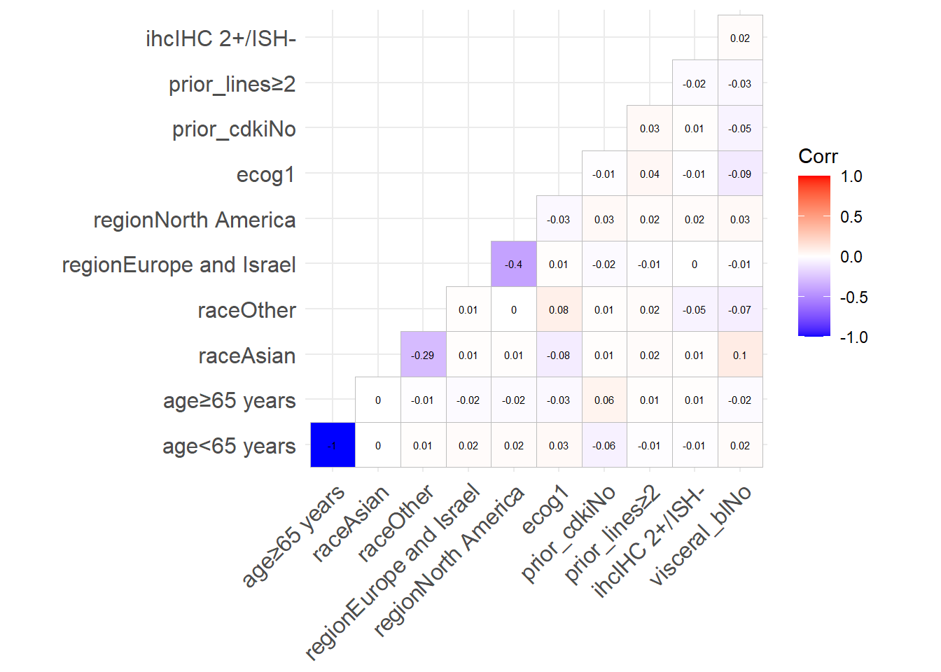

Calculation of times ⏱

OK, now we have baseline data and coefficients, we can generate survival times for our virtual patients.

To reproduce Figure S2, we need to simulate univariate interactions between all the covariates and the treatment arm.

Here, I used pivoting and joining to compute, for each patient, the sum of the coefficients corresponding to the values of their covariates.

I then use this sum, along with the coefficient for treatment arm, in the formula for a Weibull time.

I also generate a Weibull censorship time and set the end of study time to 20 months.

Similarly to the baseline data generation, this implies randomness, so I set the seed beforehand.

# HR for PFS, 0.51; 95% CI, 0.40 to 0.64; P<0.001
beta_arm = log(0.51)

add_surv_times = function(data, a=2, b=0.55, eos=Inf){
  data %>%
    pivot_longer(-c(id, arm), names_to = "variable_key", values_to = "level") |> 
    left_join(data_coef, by = c("variable_key", "level"))  |> 
    replace_na(list(coef=0, coef_rel=0)) |> # Impute missing data to 0
    summarise(
      coef_sum = sum(coef_rel),
      .by=c(id)
    ) |> 
    right_join(data, by="id") |> 
    mutate(
      arm_ttt = arm == "T-DXd",
      logw = a + b * (log(rexp(n())) - (beta_arm+coef_sum)*arm_ttt),
      time_event = exp(logw),
      time_cens = rweibull(n=nrow(data_baseline), 5, 8), #5/8 cherry-picked with KM plots
      time = pmin(time_event, time_cens, eos),
      event = time<time_cens & time<eos,
    ) |> 
    mutate(
      arm = fct_relevel(arm, "Physician's choice"),
      prior_cdki = fct_relevel(prior_cdki, "Yes"),
      ihc = fct_relevel(ihc, "IHC 1+"),
      prior_lines = fct_relevel(prior_lines, "1"),
      age = fct_relevel(age, "<65 years"),
      race = fct_relevel(race, "White", "Asian"),
      region = fct_relevel(region, "Asia", "Europe and Israel"),
      ecog = fct_relevel(ecog, "0"),
      visceral_bl = fct_relevel(visceral_bl, "Yes"),
    )
}

# set.seed(921)
set.seed(428)
data_surv = add_surv_times(data_baseline, eos=20)
data_surv

We can also generate Kaplan-Meier curves to illustrate the data.

p1=ggsurvfit(survfit(Surv(time, event) ~ arm, data=data_surv))
p2=ggsurvfit(survfit(Surv(time, event) ~ arm+ecog, data=data_surv))
p1 + p2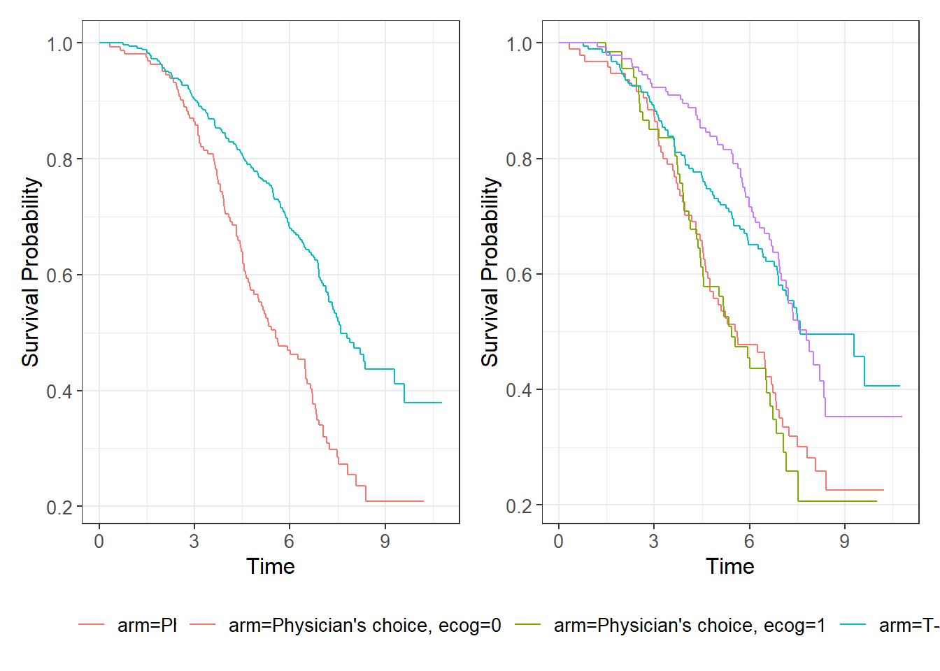

Mission completed 🚀

Hurray, we have simulated the dataset!

Now, can we reproduce the Figure S2 from our simulated data.

coef_table = function(data, exp=TRUE){
  variables = c("prior_cdki", "ihc", "prior_lines", "age", #figS2 order
                "race", "region", "ecog", "visceral_bl")
  variables |> 
    set_names() |> 
    map(~{
      data |> 
        select(everything(), value=all_of(.x)) |> 
        filter(!is.na(value)) |> 
        summarise(
          m = broom::tidy(coxph(Surv(time, event) ~ arm), 
                          conf.int=TRUE, exponentiate=exp),
          .by=value
        ) |> 
        unpack(m) |> 
        mutate(variable = .x, .before=0)
    }) |> 
    list_rbind() |> 
    mutate(variable=as_factor(as.character(variable)),
            value=fct_rev(as_factor(as.character(value)))) |> 
    arrange(variable, value)
}

coef_surv = coef_table(data_surv)
coef_surv

p = coef_surv |> 
  ggplot(aes(y=fct_rev(value), x=estimate, xmin=conf.low, xmax=conf.high)) +
  geom_point(shape="square", na.rm=TRUE) +
  geom_errorbar(width = 0.6) +
  geom_vline(xintercept=1, linetype="dashed", alpha=0.7) +
  geom_vline(xintercept=exp(beta_arm), linetype="dotted", alpha=0.6) +
  facet_grid(rows="variable", scale="free_y", ) +
  labs(x="Hazard radio", y=NULL)

fig_s2 <- png::readPNG("fig_s2_mod.png", native=TRUE)
p + fig_s2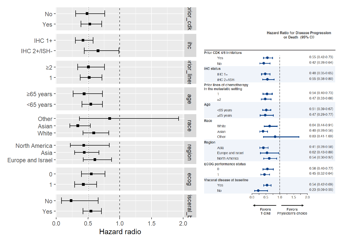

That’s not perfect, but it is close enough to play around during the course.

Post-production 🛠

Now that the proof of concept is done, the final touch will be to turn this dataset into something more real-lify, with dates instead of times.

library(lubridate)
accrual = as.Date(c("2018-12-27", "2021-12-31"))
destiny_breast04 = data_surv |> 
  mutate(date_enrolment = sort(sample(seq(ymd("2018-12-27"), ymd("2021-12-31"), by="day"), n())),
         date_end_of_study = date_enrolment + time*365.24/12,
         event_end_of_study = event,
         ) |> 
  select(id, arm, age:visceral_bl, date_enrolment, 
         date_end_of_study, event_end_of_study)
saveRDS(destiny_breast04, "destiny_breast04.rds")
destiny_breast04

Now, the resulting dataset can be downloaded from destiny_breast04.rds.

Bonus: Seed optimizations 📈

Yeah, OK, I cheated a little…

In fact, I’ve been optimizing the seeds the whole time, so that the results looks the most like the original data.

Here is how I did it.

Seed optimization on correlation

optim_correl_data = function(seed, data_fun=get_data){
  set.seed(seed)
  d = data_fun() |> select(-id, -arm)
  df_cor = 
    model.matrix(~0+., data=d) %>% 
    cor(use="pairwise.complete.obs")
  df_cor[upper.tri(df_cor)] = 0
  df_cor[abs(df_cor)==1] = 0
  sum(abs(df_cor))
}
optim_correl_data = memoise::memoise(optim_correl_data, cache=cachem::cache_disk("cache"))

cor_rslt = seq(1000) |> 
  set_names(~paste0("seed",.x)) |> 
  map_dbl(.progress=TRUE, ~{
    optim_correl_data(.x)
  })
cor_rslt[which.min(cor_rslt)] #seed517 = 1.978
#>  seed517 
#> 1.978512

Seed optimization on coefs

optim_coef_data = function(seed, fun=add_surv_times, data=data_baseline){
  set.seed(seed)
  # d = data_surv
  d = fun(data, eos=20)
  x = coef_table(d, exp=FALSE) |> 
    rename(variable_key=variable, level=value) |> 
    left_join(data_coef, by=c("variable_key", "level")) |> 
    select(variable_key, level, coef, estimate) |> 
    mutate(delta = coef-estimate, 
           delta_rel = delta/coef)
  x
}
optim_coef_data = memoise::memoise(optim_coef_data, cache=cachem::cache_disk("cache"))

coef_rslt = seq(1000) |>
  set_names(~paste0("seed",.x)) |>
  map(.progress=TRUE, ~{
    optim_coef_data(.x)
  })
coef_rslt |> map_dbl(~sum(abs(.x$delta))) |> which.min() #seed921 
#> seed921 
#>     921
coef_rslt |> map_dbl(~sum(abs(.x$delta))) |> min() #1.278669
#> [1] 1.278669

coef_rslt |> map_dbl(~sum(abs(.x$delta_rel))) |> which.min() #seed428 
#> seed428 
#>     428