What model should we use when competing risks arise?
R
code
analysis
survival
Author
Dan Chaltiel
Published
January 13, 2025
TL;DR
Fine and Gray subdistribution model is designed for prediction and should not be used for causal analysis as it yields biased estimations of Hazard Ratios.
Introduction
If you are fitting a survival analysis on an endpoint that is not death, there are chances that you will face the problem of competing risks at some point.
The most known methods to address this problem are cause-specific censoring and Fine & Gray’s subdistribution method, although multistate models are entering the game.
Competing risks arise when an individual is at risk of experiencing multiple events of events, and the occurrence of one event precludes the occurrence of the others.
For example, in clinical trials, a patient may be at risk of cancer progression (the primary event of interest) but could also die from unrelated causes before progression occurs, making progression no longer observable.
Properly accounting for competing risks is crucial, as standard survival methods like Kaplan-Meier can overestimate the probability of the event of interest by ignoring other risks that “compete” with it.
However, the 2 methods are not equivalent, and we are about to show in what.
library(tidyverse)#' Simulated dataset#' #' Simulate 2 variables `x` and `z` with normal distribution and `r` correlation,#' and 2 Weibull times depending on either `x` or `z`, then let them censor each#' other to mimic competing risks.#'#' @param n number of observations#' @param r correlation between `x` and `z`#' @param beta the true coefficient for `x` and `z`#' @param eos non-informative censoring (end of study)#' @param inf_censoring informative censoring (common risk factor for `x` & `z`)#' @param seed RNG seed#' get_df =function(n=10000, r=0.5, beta=0.5, eos=14, inf_censoring=FALSE, seed=NULL){if(!is.null(seed)) set.seed(seed) rtn =tibble(id =seq(n),# Generate a common risk factor if inf_censoring=TRUEcomrisk = inf_censoring *rnorm(n),# Generate x and z, bivariate standard normal with r=.5x =rnorm(n),z = r*x +sqrt(1-r^2)*rnorm(n),# Generate time_a (Weibull) depending on x with coefficient betalogw =2+1.5*(log(rexp(n)) - beta*x) +2*comrisk,time_a =exp(logw),# Generate time_b (Weibull) depending on z with coefficient betalogy =2+1.5*(log(rexp(n)) - beta*z)+2*comrisk,time_b =exp(logy),# *Allow events to censor each other;t =pmin(time_a, time_b, eos),event_num =case_when(t>=eos~0, time_b>time_a~1, .default=2),event =factor(event_num, 0:2, c("Censored", "Type A", "Type B")), ) rtn %>%select(id, t, event, x, z, time_a, time_b)}
Here, we have a dataset with, for each patient id, an observed time t and the event associated. The time t is either equal to the smaller time between time_a, time_b, and the administrative censoring time that we set to eos=8.
Regression models
OK, now let’s use this dataset to fit cause-specific Cox and Fine & Gray models, one of each for both Type A and Type B events:
Show the code for get_models()
library(survival)get_models =function(df, variance=TRUE){ rtn =lst(fg_a = cmprsk::crr(df$t, df$event, cbind(x=df$x, z=df$z), failcode="Type A", cencode="Censored", variance=variance),fg_b = cmprsk::crr(df$t, df$event, cbind(x=df$x, z=df$z), failcode="Type B", cencode="Censored", variance=variance),cox_a =coxph(Surv(t, event=="Type A") ~ x + z, data=df),cox_b =coxph(Surv(t, event=="Type B") ~ x + z, data=df) ) rtn}# cmprsk::crr can be long so we cache the resultget_models = memoise::memoise(get_models, cache=cachem::cache_disk("cache"))get_df = memoise::memoise(get_df, cache=cachem::cache_disk("cache"))
Informative censoring is a known problem that is difficult to adress.
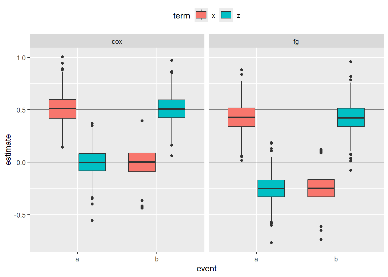
As you can see, both model are now biased. However, the cause-specific Cox model still gives less biased estimates than the Fine and Gray model.
Conclusion
Fine and Gray subdistribution model is designed for prediction and should not be used for causal analysis as it yields biased estimations of Hazard Ratios. If you intend to interpret Hazard Ratios or their p-values, you should better use cause-specific Cox models.
Bonus: Multistate models
Another possibility is to use multistate models. For time-to-event data such as ours, the MultiState Hazard (MSH) model, implemented in package survival, is pretty much adapted as it is similar to the Cox model. See the “compete” vignette for more insight.
Fitting such a MSH model for competing risks is very straightforward: you use the coxph() function with event being a factor which first level should be the censoring.
Our data is already constructed this way, so the code is:
library(survival)fit =coxph(Surv(t,event)~x+z, data=df, id=id)fit$transitions#> to#> from Type A Type B (censored)#> (s0) 4349 4260 1391#> Type A 0 0 0#> Type B 0 0 0tidy(fit) %>%arrange(term)
As expected, we get the exact same coefficients as with the 2 separate cause-specific models.
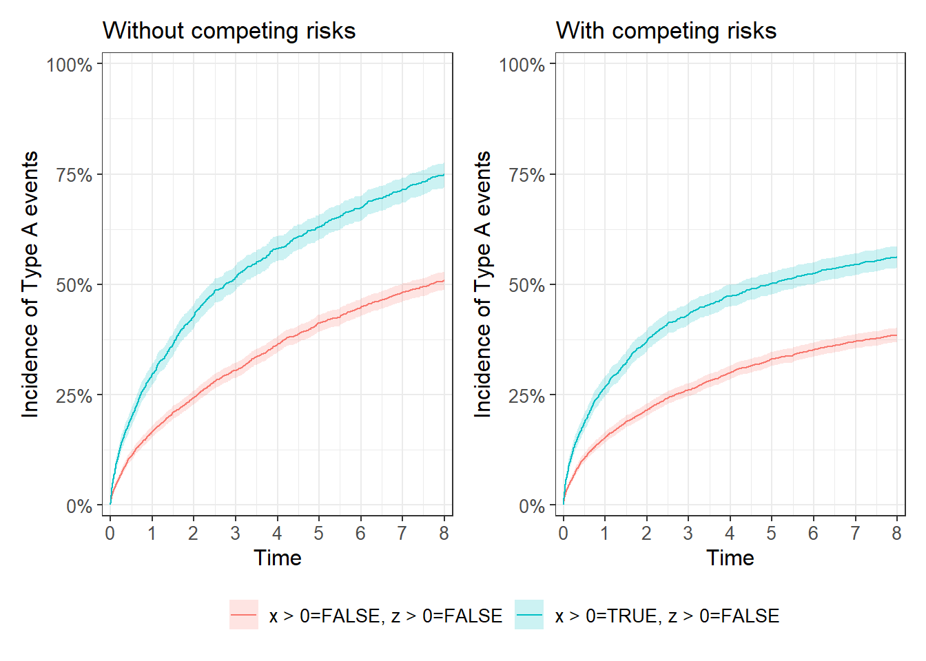
The interest about MSH models rises with plots, as the cause-specific Kaplan Meier estimator overestimates the risk in the presence of competing risks.
To illustrate this, lets binarise our x and y variables on whether they are >0.
First, you can see that mere binarisation itself introduces a large amount of bias, with x>0 being wrongly associated with Type B events, and z>0 with Type A events.
Now, we can show that the type I error is kept to the prespecified alpha=5% for CS-Cox models while it rises to 55% for F&G models!
The difference is less important for the type II error: for a true coefficient of 0.5, we have a statistical power of 98% for CS-Cox and 92% for F&G models.