Should I adjust on this one?

Introduction

Confusion bias is one of the most known and common bias that can affect our analyses. Less known is the collider bias, although its effect should not be underestimated.

When dealing with confusion bias, the usual way is to adjust on confounding variables. However, adjusting on a collider is precisely what causes the collider bias.

Tip

I highly recommend Harvard’s “Draw Your Assumptions Before Your Conclusions” free online course. It explains DAGs and uses them to illustrates all kinds of biases.

In this post, we will simulate data and illustrate how those biases happen, and how strong they can be depending on different parameters.

Scenarios

Let’s take a simple case: you want to measure the association between Y (binary) and X (continuous), and your dataset contains another variable Z (continuous) correlated to X.

We will consider 3 causal scenarios, in which we are interested in the relationship between X and Y, with X being correlated with Z:

• Scenario 1: Y is caused by X alone (regardless of Z), there is no bias.
  Example: Y is cancer, X is smoking, and Z is consumption of coffee.

flowchart LR
    X -->|?| Y[Y=1]
    Z <--> X
    style X fill:#e8f2fc,stroke:#2986e9
    style Y fill:#f4e3f3,stroke:#c160c1
    style Z fill:#dff6f4,stroke:#44d4c4

• Scenario 2: Y is caused by X and Z, there can be confounding bias and you probably should adjust on Z.
  Example: Y is cancer, X is smoking, and Z is non-healthy behaviour (e.g. measured by diet quality).

flowchart LR
    X -->|?| Y[Y=1]
    Z <--> X
    Z --> Y
    style X fill:#e8f2fc,stroke:#2986e9
    style Y fill:#f4e3f3,stroke:#c160c1
    style Z fill:#dff6f4,stroke:#44d4c4

• Scenario 3: Y is caused by X, and Z is caused by X and Y, there is a collider bias if you adjust on Z.
  Example: Y is cancer, X is smoking, and Z is pulmonary infection.

flowchart LR
    X -->|?| Y[Y=1]
    Y --> Z
    X <--> Z
    style X fill:#e8f2fc,stroke:#2986e9
    style Y fill:#f4e3f3,stroke:#c160c1
    style Z fill:#fff8e1,stroke:#ffc61b

Important

Here, I used a double arrow to note a simple association. Z could cause X, X could cause Z, or an unknown factor W could cause X and Z. This is not usual in DAGs which should be acyclical.

Simulation

To simulate this, we will need to:

1. generate datasets with the appropriate correlation structure
2. apply a logistic regression on each and save the right attributes
3. cross every possible scenario to have a good coverage of the problem

Data simulation function

OK so first, we have to build a function that can simulate a dataset along these 3 scenarios.

Disclaimer

The following code was inspired by the one published as supplemental material in the article of Paul H. Lee in Sci Rep, many thanks to the author.

This code generates:

• X as a normally distributed vector
• Z as a normally distributed vector with a fixed correlation to X.
• Y as a binary vector that represents the outcome of a logistic regression influenced by X with coefficient beta_x (and Z with coefficient beta_z in the “confounding” scenario).

The only exception is in the “collider” scenario, where Z is generated (using this code) so it has a fixed correlation to both X and Y.

library(tidyverse)

invlogit = function(x) 1/(1+exp(-x)) #inverse-logit function

data_sim = function(N, correlation, beta_x=0.2, beta_z=0.2, 
                    type=c("no_bias", "confounding", "collider"),
                    seed=NULL){
  if(!is.null(seed)) set.seed(seed)
  type = match.arg(type)
  x = rnorm(N)
  if(type=="no_bias"){
    # Y is computed from X only: Z is an unrelated variable (noise)
    z = correlation*x + sqrt(1-correlation^2) * rnorm(N)
    y = rbinom(N, 1, 1-invlogit(-beta_x*x))
  } else if(type=="confounding"){
    # Y is computed from both X and Z: Z is a common cause (confounding bias)
    z = correlation*x + sqrt(1-correlation^2) * rnorm(N)
    y = rbinom(N, 1, 1-invlogit(-beta_x*x -beta_z*z))
  } else if(type=="collider"){
    # Z is computed from both X and Y: Z is a collider (collider bias)
    y = rbinom(N, 1, 1-invlogit(-beta_x*x))
    z = rcorrelated(x, y, correlation) #rcorrelated is a custom function
  }
  
  tibble(x,z,y)
}

show_cor = function(m) {m=round(cor(m), 3);m["z","z"]=NA;m[c("z","y"),c("x","z")]}

The correlations depend on the effect of X and Z on Y, but we can see that the fixed correlations are respected:

df = data_sim(1000, correlation=0.3, beta_x=9, beta_z=9, type="no_bias", seed=42)
show_cor(df) #cor(X,Z)=0.3
#>       x     z
#> z 0.313    NA
#> y 0.776 0.236
df = data_sim(1000, correlation=0.3, beta_x=9, beta_z=9, type="confounding", seed=42)
show_cor(df) #cor(X,Z)=0.3
#>       x     z
#> z 0.313    NA
#> y 0.634 0.639
df = data_sim(1000, correlation=0.3, beta_x=9, beta_z=9, type="collider", seed=42)
show_cor(df) #cor(X,Z)=cor(Y,Z)=0.3
#>       x   z
#> z 0.300  NA
#> y 0.777 0.3

Logistic regressions

OK, we know how to make datasets, now let’s draw a bunch of them and make some regression so we can see the effect of adjusting on Z.

In the following function, we generate n_sim datasets and for each we fit:

• one bare logistic model y~x
• and one adjusted logistic model y~x+z.

Then we return the coefficient, standard error, and p-value of each variable of each model.

Tip

As running all these scenarios takes a significant amount of time, I’m using {memoise} to cache the result of each simulation.

pval = function(beta, se) 2-2*pnorm(abs(beta)/se) #helper to calculate the p-value

simulate = function(n_sim, sample_size, correlation, 
                    beta_x=0.2, beta_z=0.2, 
                    type=c("no_bias", "confounding", "collider"),
                    seed=NULL, verbose=TRUE){
  if(!is.null(seed)) set.seed(seed)
  if(verbose) {
    message(glue::glue("- Simulating: n_sim={n_sim}, sample_size={sample_size}, correlation={correlation}, beta_x={beta_x}, beta_z={beta_z}, type={type}, seed={seed} \n\n"))
  }
  
  seq(n_sim) %>% 
    map(~{
      df = data_sim(N=sample_size, correlation=correlation, 
                    beta_x=beta_x, beta_z=beta_z, type=type, 
                    seed=NULL)
      m_bare = glm(y~x,   family=binomial(link="logit"), data=df)
      m_adju = glm(y~x+z, family=binomial(link="logit"), data=df)
      
      tibble(
        simu  = .x,
        seed = seed,
        # data  = list(df), #makes the final object too heavy
        sample_size = sample_size, correlation = correlation,
        beta_x = beta_x, beta_z = beta_z, type = type, 
        m_bare_x_coef = coef(m_bare)["x"],
        m_bare_x_se = sqrt(vcov(m_bare)["x","x"]),
        m_bare_x_p = pval(m_bare_x_coef, m_bare_x_se),
        m_adju_x_coef = coef(m_adju)["x"],
        m_adju_x_se = sqrt(vcov(m_adju)["x","x"]),
        m_adju_x_p = pval(m_adju_x_coef, m_adju_x_se),
        m_adju_z_coef = coef(m_adju)["z"],
        m_adju_z_se = sqrt(vcov(m_adju)["z","z"]),
        m_adju_z_p = pval(m_adju_z_coef, m_adju_z_se),
      )
    }, .progress=n_sim*sample_size>1e5) %>% 
    list_rbind()
}

simulate = memoise::memoise(simulate, cache=cachem::cache_disk("cache/logistic_adj"), 
                            omit_args="verbose")

Just to be sure, with 1000 reps of 200 observations with a correlation of 0, we get the correct coefficient for beta_x with a quite decent precision:

sim1 = simulate(n_sim=1000, sample_size=200, beta_x=1, correlation=0,
                type="no_bias", seed=42)
sim1 %>% 
  summarise(n_sim=n(), m_bare_x_coef=mean(m_bare_x_coef))

Application: gridsearch

Using expand.grid(), we can now design various scenarios, and then use simulate() on each.

Here, I’m considering a lot of possibilities, so this will take a fair amount of time to compute the first time. Thanks to memoise though, the next times will take a few ms only!

#generic scenarios
scenarios1 = expand_grid(
  sample_size = c(200, 500, 1000), 
  correlation = seq(0, 0.5, by=0.1),
  beta_x = c(0.2),
  beta_z = c(0.2),
  type = c("no_bias", "confounding", "collider")
) 

#bias-exploring scenarios
scenarios2 = expand_grid(
  sample_size = c(500), 
  correlation = seq(0, 0.5, by=0.1),
  beta_x = c(0, 0.2),
  beta_z = seq(0, 0.5, by=0.1),
  type = c("confounding", "collider")
) 

scenarios = bind_rows(scenarios1, scenarios2) %>% distinct()

set.seed(42)
sim_all = 
  scenarios %>% 
  mutate(scenario = row_number(), .before=1) %>% 
  rowwise() %>% 
  mutate(
    sim = {
      message("Computing scenario ", scenario, "/", nrow(scenarios), "\n", sep="")
      list(simulate(n_sim=1000, sample_size=sample_size, correlation=correlation, 
                    beta_x=beta_x, beta_z=beta_z,
                    type=type, seed=NULL, verbose=TRUE))
    }
  ) %>% 
  ungroup()

saveRDS(sim_all, "logistic_adj.rds")

There we are, one row per scenario:

nrow(sim_all)
#> [1] 186

Tip

I’m saving this in the file logistic_adj.rds, so you can use it directly if you want to play with these results.

Results: coefficients

At last, we can explore our results and make some plots!

Data

First, we have to wrangle out simulations into a workable dataframe. This implies summarising each simulation (here I’m using mean, sd, median, and quantiles on the X coefficient), then applying a bit of dplyr and tidyr magic:

df_coef =
  sim_all %>% 
  rowwise() %>% 
  mutate(sim = summarise(sim, 
                         across(c(m_bare_x_coef, m_adju_x_coef), 
                                lst(mean, sd, median, 
                                    pc25=~quantile(.x, 0.25), pc75=~quantile(.x, 0.75))))) %>% 
  unpack(sim) %>% 
  mutate(across(matches("m_...._._coef"), 
                .fns=~(.x-beta_x)/beta_x, 
                .names="{.col}_error")) %>% 
  pivot_longer(matches("m.*_x_"),
               names_pattern=c("m_(.*)_x_(.*)"), names_to=c("model",".value"),
               names_transform=\(x) paste0("x_",x)
  ) %>% 
  mutate(
    type2 = factor(type, levels=c("no_bias", "confounding", "collider"),
                   labels=c("No bias", "Confounder", "Collider")),
    model2 = factor(model, levels=c("x_bare", "x_adju"), 
                    labels=c("Bare model", "Adjusted model")),
    scenario = paste(type2, model2, sep=" - ") %>% fct_rev(),
    effect_z = paste0("Coef(Z)=",beta_z)
  ) 

datatable(df_coef, class='nowrap display')

Error on X depending on scenario

Now, let’s plot the error on the coefficient for X, for each sample size (color) and scenario (column), and compare the bare model with the adjusted model (rows).

pd = position_dodge(width = .05)
capt = "The dots and whiskers represent the median and the 25th and 75th percentiles of the X coefficient among the N simulated trial replicates." %>% str_wrap(width=nchar(.)/2)
df_coef %>% 
  filter(beta_x==0.2 & beta_z==0.2) %>%
  ggplot() +
  aes(x=correlation, color=factor(sample_size), fill=factor(sample_size)) +
  geom_pointrange(aes(y=x_coef_median_error, ymin=x_coef_pc25_error, ymax=x_coef_pc75_error), 
                  position=pd) +
  geom_hline(yintercept=0, alpha=0.3) +
  facet_wrap(model2~type2, scales="free_y") +
  scale_x_continuous(breaks=scales::breaks_width(0.1), labels=scales::label_percent()) +
  scale_y_continuous(labels=scales::label_percent()) +
  labs(x="Correlation between X and Z", y="Relative error on X coefficient", 
       color="Sample size", fill="Sample size",
       caption=capt)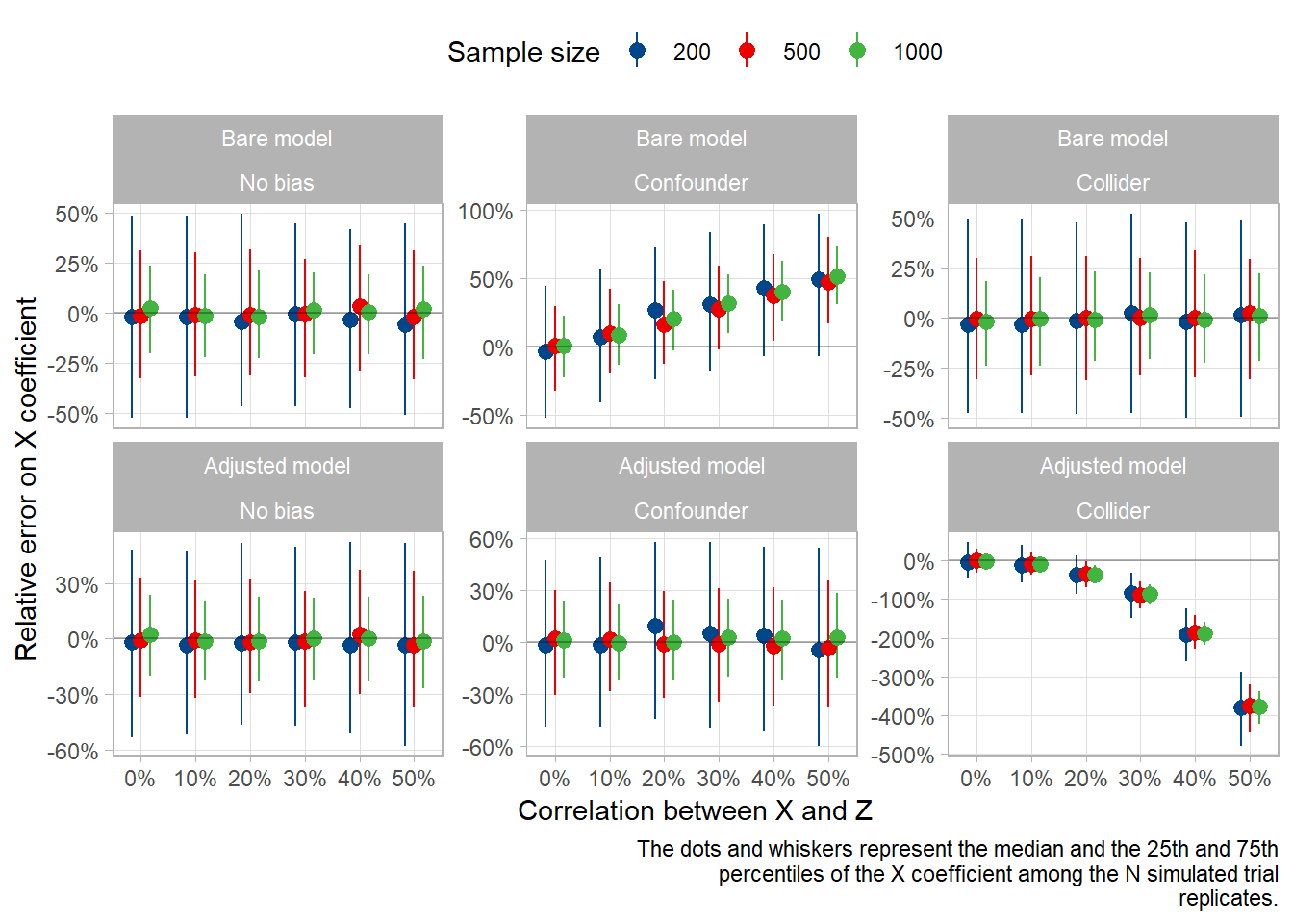

As you can see, the error is around 5% in most scenarios, except for 2:

• When there is a confounder that we don’t adjust on (overestimation in this case)
• When there is a collider that we adjust on (underestimation in this case)

The error is directly dependant on the correlation between X and Z, with a linear trend for the non-adjusted confounder and a non-linear trend for the adjusted collider.

Note that we should probably not extrapolate on the functional form of this latter non-linear trend, as it is most likely dependant on the correlation structure in our simulation rather than on the type of bias. In our collider scenario, Z is correlated with both X and Y. In the original paper, the author used z <- rnorm(sample_size) + cor_x_z*x + y, and it didn’t show this kind of pattern.

Error on X depending on effect of Z

If we fix coefficient beta_x to 0.2, we can now vary beta_x to see the difference in bias magnitude.

df_coef %>% 
  filter(beta_x==0.2, sample_size==500) %>%
  filter(scenario=="Confounder - Bare model" | scenario=="Collider - Adjusted model") %>% 
  ggplot() +
  aes(x=correlation) +
  geom_col(aes(y=x_coef_mean_error), 
           position=pd, alpha=0.1) +
  geom_pointrange(aes(y=x_coef_median_error, ymin=x_coef_pc25_error, ymax=x_coef_pc75_error), 
                  position=pd) +
  geom_hline(yintercept=0, alpha=0.3) +
  facet_grid(scenario~effect_z, scales="free_y") +
  scale_x_continuous(breaks=scales::breaks_width(0.1), labels=scales::label_percent()) +
  scale_y_continuous(labels=scales::label_percent()) +
  labs(x="Correlation between X and Z", y="Relative error on X coefficient", 
       color="Sample size", fill="Sample size",
       caption=capt)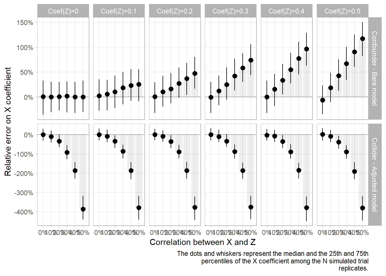

As expected, in both cases, there is more bias when the confounder/collider Z has a greater effect on Y than X.

Results: p-values

Data

Same as before, we need to wrangle our data into a workable dataframe. Here, I’m using prop.test to get the confidence interval of the proportion of significant p-values at alpha=5%. Then I’m painfuly unnesting and unpacking into nice columns.

We set the hypothesis to H0 or H1 depending on whether beta_x==0 so that we can see the effect on risks alpha and beta.

df_pval =
  sim_all %>% 
  rowwise() %>% 
  mutate(sim = summarise(sim, across(ends_with("_p"), ~{
    x = prop.test(sum(.x<0.05), length(.x))
    tibble(mean=x$estimate, mean_check=mean(.x<0.05), inf=x$conf.int[1], sup=x$conf.int[2])
  }))) %>% 
  unnest(sim) %>% 
  unpack(everything(), names_sep="_") %>% 
  pivot_longer(matches("_p_"),
               names_pattern=c("m_(.*)_(.)_p_(.*)"), 
               names_to=c("model","term",".value"),
               names_transform=\(x) paste0("pval_", x),
  ) %>% 
  mutate(
    type2 = factor(type, levels=c("no_bias", "confounding", "collider"),
                   labels=c("No bias", "Confounder", "Collider")),
    model2 = factor(model, levels=c("pval_bare", "pval_adju"),
                    labels=c("Bare model", "Adjusted model")),
    scenario = paste(type2, model2, sep=" - ") %>% fct_rev(),
    hypothesis = ifelse(beta_x==0,"H0", "H1"),
    effect_z = paste0("Coef(Z)=",beta_z)
  )

Error on p-values-driven decisions: confusion bias

As we observed above, the confusion bias depends on the correlation between X and Z and on the strength of the effect of Z, Coef(Z).

Let’s plot the proportion of significant values (alpha=5%) for X when Coef(X)=0 (H0) and when Coef(X)=0.2 (H1), and see how it depends on those variables.

df_pval %>%
  filter(term=="pval_x") %>% #we don't really care about Z significance
  filter(sample_size==500) %>% #these sims were made on N=500 only
  filter(scenario=="Confounder - Bare model") %>%
  ggplot(aes(x=correlation, y=pval_mean, ymin=pval_inf, ymax=pval_sup, color=factor(beta_z))) +
  geom_pointrange(size=0.3) + geom_line() +
  facet_wrap(~hypothesis) +
  # facet_grid(hypothesis~beta_z) + #this plot is nice too
  labs(x="Correlation between X and Z", y="Proportion of p-value<0.05 for X coefficient", 
       color="Coef(Z)") +
  guides(color=guide_legend(nrow=1,byrow=TRUE))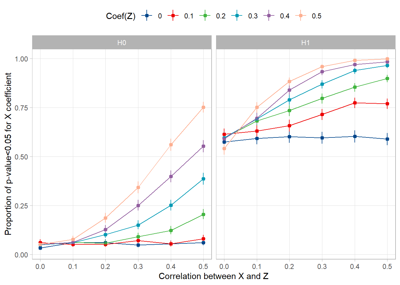

The dots and whiskers represent the proportion of significant values over the 1000 simulations and its very small 95% confidence interval.

Under H0 (left panel), when Coef(Z)=0, i.e. when there is no confusion bias, the proportion of significant values is stable at 5%. This is expected from the pre-specified alpha, and serves as internal validation. Then, the more you increase Coef(Z) and Cor(X,Z), the more false positives you get: the alpha risk increases.

Under H1 (right panel), when Coef(Z)=0, the proportion of significant values is stable at a value that represents the power of the test when there is no confusion bias. Then, the more you increase Coef(Z) and Cor(X,Z), the more true positives you get: the test is overpowered. Of course this is a far less problematic issue than the one above.